Qual: Feasibility Legwork

2010 July 19

(Second deadline: also blown, but no slippage relative to the previous one.)

Can I reasonably expect to accomplish what I’m setting out to accomplish? This post will present some of the quantitative legwork needed to answer that question.

Cyg X-3🔗

There are two key feasibility issues for the Cyg X-3 project in my view:

1. Can we successfully process the data?
2. Will the dataset allow us to do interesting science?

1. We can successfully image the data:

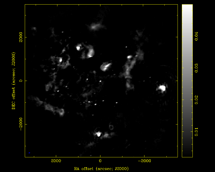
It’s a complicated region, but we can clearly get something decent out, and we can detect Cyg X-3 nicely.

But the actual dataset that we’re looking to create is a time-series of flux measurements for Cyg X-3. Can we obtain sufficiently precise and high-cadence fluxes? This is, in a sense, a moving-goalpost problem: we can always scale back our goals for precision and/or cadence, and sooner or later they’ll be achieved. It might bode ill for the well-posedness of the scientific problem that there isn’t any particular cutoff at which we think it’ll become impossible to obtain interesting results, though if we have to scale back so much that our dataset will be very similar to existing radio datasets, that’s a bad sign.

From analysis of some of the images that I’ve made of the Cygnus and GC regions, it appears that I can expect to achieve a “noise factor” (NF) of 10 mJy sqrt(hr) / bm for one correlator — that is, a 1-hr integration should give me an RMS noise of 10 mJy/bm, a 10-minute integration about 25 mJy/bm, etc. Still considering a single correlator, this is about twice what I see on long integrations on a calibrator, which involve much less crowded fields but are quite possibly dynamic-range-limited (DR ~ 2000-3000 in the images I was looking at). This is also about 15 times the naive expectation you get based on the performance of the individual antpols (ignoring that data get flagged, that we don’t get all baselines, etc.) This number is definitely conservative, and could be improved by improvements in the analysis pipeline, calibration, array performance, etc. I actually haven’t done a whole lot of dual-correlator work, so discounting a little bit you’d estimate having a dual-correlator NF of 8 or so, and with other analysis improvements, an NF of 5 seems quite achievable.

But let’s proceed with the current figure of NF = 10. Since Cyg X-3 is about 100 mJy, that means that if we chunk our data into 10-minute intervals we get ~4-sigma detections in each chunk, which seems good. This also yields about 30 samples per 4.8-hr orbit, which is also good.

The main limiting factor here is unknown systematics in the data. From UV modeling work, I know they’re in there, and they seem to be present at levels comparable to the brightness of Cyg X-3. (This is what I get if I time average over all baselines and pols and look at the resulting amplitudes, which seem as if they might have some continuity to them.) This could be a very big deal, but it’s hard to assess — maybe I’ll figure out how to make the fit residuals go away entirely, maybe I’ll have to figure out a way to live with them. I postpone deeper consideration of this to the next feasibility post.

2. Then there’s the question of whether our dataset will actually yield any scientifically interesting results. This is the trickiest one because it’s really hard to answer before we actually have nice radio and X-ray lightcurves to look at. To provide some grist for consideration, here’s a simple graphic showing spans of ATA observations, X-ray observations, and outbursts by Cyg X-3. It’s not at all legible in its current form but it’s good enough to show a few important points.

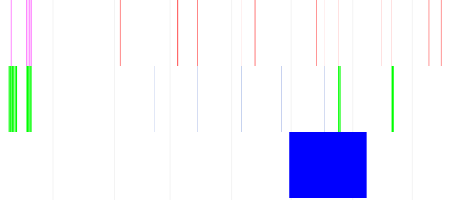
The X axis is time, with the vertical lines spanning the entire plot showing the beginnings of months, with the leftmost line denoting January 1 2010. The top row of shorter marks shows selected ATA observations of Cyg X-3: ones at useful 3 GHz in red, ones at frustrating 1.4 GHz in purple. I’m only showing observing runs that either have 1) a lot of time spent on X-3 or 2) close proximity to an X-ray observation. We have runs every few days throughout this entire timespan, though not all of them have significant time on X-3. The second show shows X-ray observations: INTEGRAL in green, RXTE in sea-foam-ish. The third row shows a period of outburst that Cyg X-3 went through. If you zoom in, you can see that we have 5 epochs of (near) simultaneous radio/X-ray observations, even if you don’t count the lengthy epochs at 1.4/2.01 GHz in December 2009. Two of those are during the general outburst period. The backing data for this plot, with precise timing information canonicalized to MJD, are in /cosmic1/pkwill/ata/cygx3/extra-obs.txt.

I think this is encouraging for the notion that if we can reduce the data, we’ll have interesting comparisons to make.

AGCTS🔗

There are three key feasibility issues for the AGCTS:

1. Can we successfully process the data?
2. Can we expect to find transients or put interesting constraints on their rates?
3. Will this be an improvement on existing work?

1. As with Cyg X-3, we can image the data. This is made “interesting” with the summer 2010 AGCTS dataset because we have very consistent hour angle coverage for all of the fields, which allows nice interepoch comparisons but makes for lousy images. We hope to be working in the UV domain as much as possible, so hopefully this will turn out to be a good thing overall.

Compared to Cyg X-3, the only additional difficulty that I can think of with imaging the GC is that Sgr A* is much brighter than anything in the Cygnus field. (Cyg A typically comes in a 40 mJy.) In one sample dataset it came in at ~45 Jy, and the image had a dynamic range of … ~400. That’s certainly a challenge. Hopefully, we can get some dedicated observations with good hour angle coverage, use those to develop a high- quality model, and be able to get much better results than we do now with short observations for which Sgr A* is significant.

2/3. Talking about expected transient rates and comparing to previous work are closely connected, because there are a lot of different ways to assess transient rates and different surveys probe different aspects of these rates, so you end up with more-or-less a 1:1 map between a particular rate measurement and a particular survey in the literature.

Ignoring all of the data at 1.43/2.01 GHz, there are currently (2010 Jul 16) 35 AGCTS epochs after 2010 Apr 28, when we switched frequencies. In that dataset we currently have 688 source scans at 3.14 GHz for a total of 115 hours of data, with a presumably comparable number at 3.04 GHz. The effective area of each scan is almost precisely 1 sq.deg out to FWHM. The mean scan duration is 604s and the median scan duration is 420s, leading to expected RMS fluxes of 25 or 30 mJy/bm, respectively, for a single correlator. To some extent, that’s the capsule summary of the survey: 1 sq.deg x 115 hr x ~28 mJy/bm.

We can also consider the survey speed of various instruments used for radio transient surveys. The relevant ones here are ATA/3.14 GHz (me), GMRT/0.235GHz (Hyman+), VLA/0.33GHz (Hyman+), and VLA/4.86 GHz (Becker+). A figure of merit for the survey speed of a particular radio instrument is:

Using deg, m, and K, I get ATA/3.14: 284, GMRT/0.235: 278784, VLA/0.33: 65373, VLA/4.86: 2822. Sadly these are not typos. What these numbers come down to is that the ATA gets murdered in effective area. (Not-ATA notebook #1 p. 64.)

There are several ways to make up for this. One is time-on-target: AGCTS has 115 hours so far and is on track for perhaps 200, assuming that we accomplish nothing with the ~200 additional hours of 1.43/2.01 GHz data. The 2008 Hyman+ paper reported about 66 hours of observing. The CORNISH survey, the intermediate version of which the Becker+ work is based, was allocated 400h; it appears that the Becker+ work was performed with about half of the data in, so call that 200h. We beat Hyman+ on time but not by nearly a sufficient margin to make up for our inferior effective area.

But AGCTS is exploring a different region of parameter space than Hyman+. We’ll be sensitive to brighter, and thus rarer, events. Our total area covered is much larger than Hyman+, giving us an edge for things that in particular are rare in an areal sense. (There’s also rarity in a duty-cycle sense.) We’re comparable to the Becker+ work in area, and we have less time, and our sensitivity is much poorer … but at least we’re focusing on the GC while they’re looking elsewhere in the plane, and their work in fact indicates that the areal transient rate goes up nontrivially as you get closer to the GC.

Our cadence is more rapid than that of Hyman+ or Becker+. We’ll revisit the same area once every few days in most cases, whereas Hyman+ operates on a monthly basis. So our hope is that there will be bright, brief transients that last on ~week timescales.

There’s also the question of spectral index. Obviously, relative to Hyman+ we’ll be more sensitive to flat/inverted-spectrum sources, while relative to Becker+ we’ll be more sensitive to normal/steep-spectrum sources. Hyman+ reports steep spectral indices for some of their events, alpha ~ -2, but those results seem a bit sketchy. (I think they report alpha ~ -6 for one event.) Becker+ see spectral indices ranging from -3 to 2 with a median of ~-1, which is encouraging. If the Hyman+ sources really do have somewhat steep spectra, we will basically be unable to see them.

I think the positive spin on all this is that we’ll be carving out a very novel chunk of parameter space. We have an intermediate frequency, a high cadence, a large area, and low sensitivity. If there are bright, flat-spectrum transients that last about a week, we’ll own them.

This conclusion also implies that it’s hard to confidently draw conclusions from published transient rates. Despite the large difference in observing frequency, the most directly comparable survey is probably that of Hyman et al. They have found several sources in ~100 hours of observing (adding in older VLA observations that found the Burper and their first source) with typical fluxes of ~100 mJy. We’ll have somewhat more time and somewhat worse sensitivity, but are a fairly different cadence and a very different frequency. Whether we’d expect to find something depends strongly on the population of transient sources, so, conversely, whether we find anything will provide useful information on the population of transient sources.